资料收集：

google搜索或在生信技能树和生信菜鸟团搜索WGCNA ，能找到很多教程，下面列出几个中文教程和英文教程，强烈推荐中文教程1和英文教程3。

1. 一文学会WGCNA分析

2. 学习WGCNA总结

3. Tutorials for the WGCNA package

• WGCNA Background and glossary

• Data input and cleaning

• Network construction and module detection

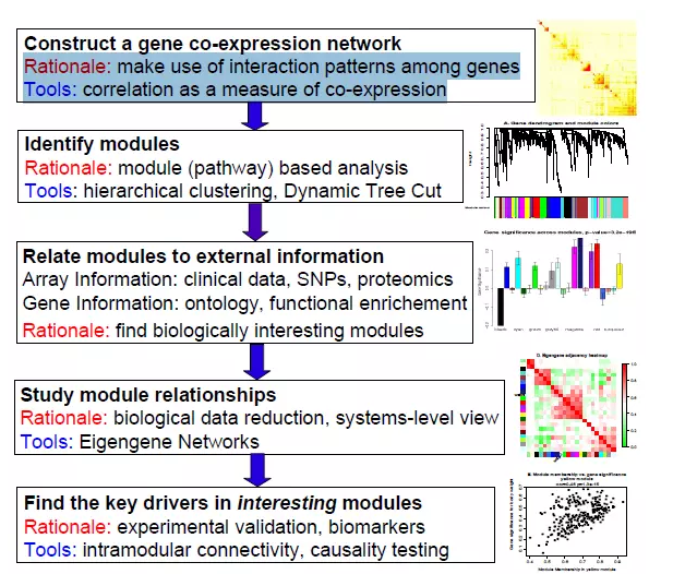
• Relating modules to external information and identifying important genes

• Interfacing network analysis with other data such as functional annotation and gene ontology

• Network visualization using WGCNA functions

• Exporting a gene network to external visualization software

背景知识

基本概念

WGCNA(weighted correlation network analysis)加权基因共表达网络分析, 用于提取与性状或临床特征相关的基因模块，解析基础代谢途径，转录调控途径、翻译水平调控等生物学过程。
WGCNA适合于复杂的数据模式，推荐5组以上的数据，如：
不同器官、组织类型发育调控；
同一组织不同时期发育调控；
非生物胁迫不同时间点应答；
病原物侵染后不同时间点应答。

基本步骤：

WGCNA分为表达量聚类分析和表型关联两部分，具体步骤包括基因之间相关系数的计算，共表达网络的构建，筛选特定模块，模块与性状关联，核心基因的筛选。

Overview of a typical WGCNA analysis.

术语：

Co-expression weighted network: 是一个无向有权重（undirected, weighted）的网络。“无权重（unweighted network）”,基因与基因之间的相关度只能是0或者1,0表示两个基因没有联系，而1表示有。“有权重（weighted network）”基因之间不仅仅是相关与否，还记录着它们的相关性数值，数值就是基因之间的联系的权重(相关性)。
Module:（模块）指表达模式相似的基因聚为一类，这样的一类基因称为模块。
Connectivity:指一个基因与网络中其他基因的相关性程度。
Eigengene（eigen- +‎ gene）：基因和样本构成的矩阵
Module eigengene E: 一个模块中的主成分
Hub gene:
Gene signicance GS:
Module signicance:

分析流程

WGCNA输入文件需要一个表达矩阵，最好是RPKM或其他归一化好的表达量；同时需要提供临床信息或者其它表型信息。

STEP1: 输入数据的准备

表达矩阵可以从作者GitHub下载 https://github.com/DChenABLife/RhesusLncRNA，这里只下载lncRNA的表达矩阵(https://github.com/DChenABLife/RhesusLncRNA/blob/master/All_sample_LncRNA_exp_RPKM.xlsx), 因为这里的表达矩阵文件是Excel格式的，需要转为csv格式方便后续用R处理，可以直接打开这个excel文件，然后另存为csv格式即可。

读入原始表达数据

原始数据包含64个样本，9904个lncRNA表达量，其中第一列是lncRNA_ID,第66列是Annotation。

setwd("G:/My_exercise/WGCNA/")
lncRNAexpr <- read.csv("All_sample_LncRNA_exp_RPKM.csv",sep=",",header = T)
head(lncRNAexpr)
dim(lncRNAexpr)#[1] 9904   66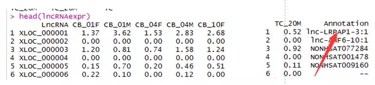

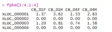
rawdata

重命名数据列表，行名和列名

##去掉Annotation这列fpkm <- lncRNAexpr[,-66]
head(fpkm)##重命名行名和列名rownames(fpkm)=fpkm[,1]
fpkm=fpkm[,-1]
fpkm[1:4,1:4]

fpkm

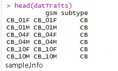
准备表型信息

这里有64个样本，包含猕猴脑不同空间区域，不同发育时期，以及性别，因为每个样本都交叉包含着三种不同的信息，如果选择全部表型信息，我试了试，后续的模块和性状完全看不清关系，所以我这里仅选择脑不同区域的表型信息,包括CB、DG、PFC、PCC、CA1、OC、PC、TC。

##Sample Infosubname=sapply(colnames(fpkm),function(x) strsplit(x,"_")[[1]][1])
datTraits = data.frame(gsm=names(fpkm),
                       subtype=subname)
rownames(datTraits)=datTraits[,1]
head(datTraits)

下载并载入WGCNA包

source("http://bioconductor.org/biocLite.R")#biocLite(c("AnnotationDbi", "impute", "GO.db", "preprocessCore")) ##如果已经下载过了，这里就不用下载biocLite("WGCNA")
library(WGCNA)

行列转置

WGCNA针对的是基因进行聚类，而一般我们的聚类是针对样本用hclust即可，也就是说要转置为行名是sample,列名是gene。

RNAseq_voom <- fpkm 
WGCNA_matrix = t(RNAseq_voom[order(apply(RNAseq_voom,1,mad), decreasing = T)[1:5000],])
datExpr <- WGCNA_matrix  ## top 5000 mad genesdatExpr[1:4,1:4]

datExpr

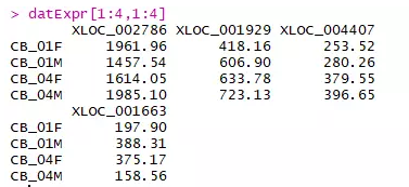
确定临床表型与样本名字

sampleNames = rownames(datExpr);
traitRows = match(sampleNames, datTraits$gsm)  
rownames(datTraits) = datTraits[traitRows, 1]

datExpr和datTraits准备好后，接下来就是构建基因网络，鉴定模块。网络构建有三种方法：1）一步法构建网络；2）多步法构建网络；3）block-wise构建网络（主要针对大数据集）。下面的介绍的步骤是一步法构建网络。

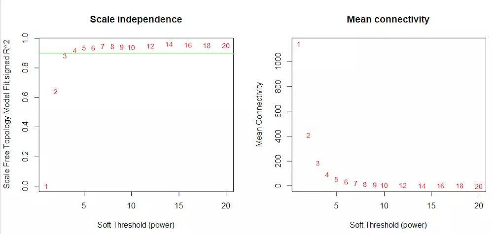
STEP2：确定最佳soft-thresholding power

选择合适“软阀值（soft thresholding power）”beta

Constructing a weighted gene network entails the choice of the soft thresholding power  to which co-expression similarity is raised to calculate adjacency.

用到的函数是pickSoftThreshold

# Choose a set of soft-thresholding powerspowers = c(c(1:10), seq(from = 12, to=20, by=2))# Call the network topology analysis functionsft = pickSoftThreshold(datExpr, powerVector = powers, verbose = 5)# Plot the results:par(mfrow = c(1,2));
cex1 = 0.9;# Scale-free topology fit index as a function of the soft-thresholding powerplot(sft$fitIndices[,1], -sign(sft$fitIndices[,3])*sft$fitIndices[,2],
     xlab="Soft Threshold (power)",ylab="Scale Free Topology Model Fit,signed R^2",type="n",
     main = paste("Scale independence"));
text(sft$fitIndices[,1], -sign(sft$fitIndices[,3])*sft$fitIndices[,2],
     labels=powers,cex=cex1,col="red");# this line corresponds to using an R^2 cut-off of habline(h=0.90,col="green")# Mean connectivity as a function of the soft-thresholding powerplot(sft$fitIndices[,1], sft$fitIndices[,5],
     xlab="Soft Threshold (power)",ylab="Mean Connectivity", type="n",
     main = paste("Mean connectivity"))
text(sft$fitIndices[,1], sft$fitIndices[,5], labels=powers, cex=cex1,col="red")#选择beta值best_beta=sft$powerEstimate#> best_beta[1] 3

最佳beta值是3。

Soft Threshold

STEP3: 一步法构建共表达矩阵

一步法构建网络，power=sft$powerEstimate=3,mergeCutHeight是合并模块阈值的一个参数。

net = blockwiseModules(datExpr, power = sft$powerEstimate,
                       maxBlockSize = 6000,TOMType = "unsigned", 
                       minModuleSize = 30,reassignThreshold = 0, mergeCutHeight = 0.25,
                       numericLabels = TRUE, pamRespectsDendro = FALSE,
                       saveTOMs = TRUE,
                       saveTOMFileBase = "AS-green-FPKM-TOM",
                       verbose = 3)

STEP4:模块鉴定及可视化

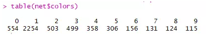
模块鉴定

table(net$colors) 可以看总共有多少模块，每个模块的大小，这里共有9个模块，从1-9每个模块的大小是递减的，从2254-115，0表示这些基因不在所有模块内。

table(net$colors)

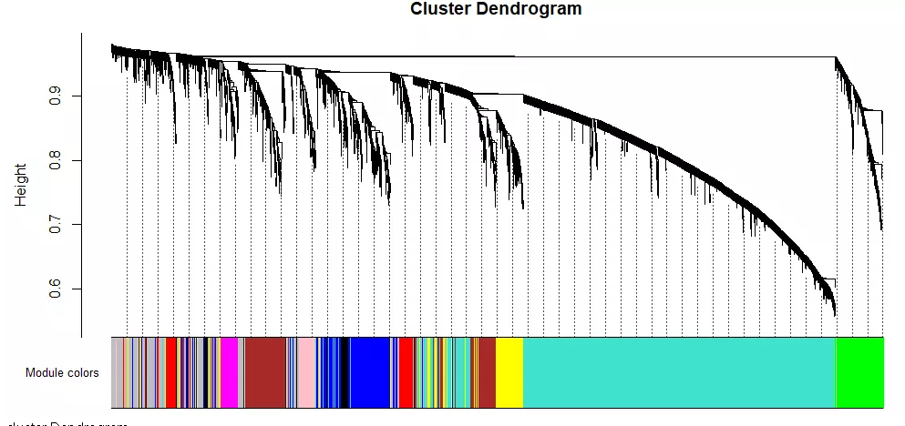
可视化

# Convert labels to colors for plottingmergedColors = labels2colors(net$colors)
table(mergedColors)# Plot the dendrogram and the module colors underneathplotDendroAndColors(net$dendrograms[[1]], mergedColors[net$blockGenes[[1]]],                    "Module colors",
                    dendroLabels = FALSE, hang = 0.03,
                    addGuide = TRUE, guideHang = 0.05)## assign all of the gene to their corresponding module ## hclust for the genes.

cluster Dendrogram

#明确样本数和基因数nGenes = ncol(datExpr)
nSamples = nrow(datExpr)#首先针对样本做个系统聚类树datExpr_tree<-hclust(dist(datExpr), method = "average")
par(mar = c(0,5,2,0))
plot(datExpr_tree, main = "Sample clustering", sub="", xlab="", cex.lab = 2, 
     cex.axis = 1, cex.main = 1,cex.lab=1)## 如果这个时候样本是有性状，或者临床表型的，可以加进去看看是否聚类合理#针对前面构造的样品矩阵添加对应颜色sample_colors <- numbers2colors(as.numeric(factor(datTraits$subtype)), 
                                colors = c("grey","blue","red","green"),signed = FALSE)## 这个给样品添加对应颜色的代码需要自行修改以适应自己的数据分析项目。#  sample_colors <- numbers2colors( datTraits ,signed = FALSE)## 如果样品有多种分类情况，而且 datTraits 里面都是分类信息，那么可以直接用上面代码，##当然，这样给的颜色不明显，意义不大。#构造10个样品的系统聚类树及性状热图par(mar = c(1,4,3,1),cex=0.8)
plotDendroAndColors(datExpr_tree, sample_colors,
                    groupLabels = colnames(sample),
                    cex.dendroLabels = 0.8,
                    marAll = c(1, 4, 3, 1),
                    cex.rowText = 0.01,
                    main = "Sample dendrogram and trait heatmap")

Sample dendrogram and trait heatmap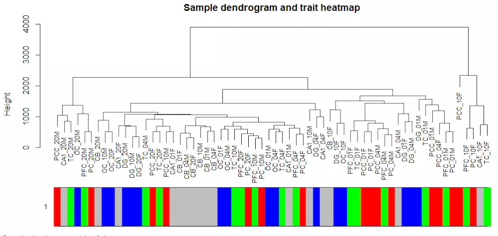

STEP5:模块和性状的关系

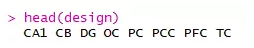
design=model.matrix(~0+ datTraits$subtype)
colnames(design)=levels(datTraits$subtype)
moduleColors <- labels2colors(net$colors)
# Recalculate MEs with color labelsMEs0 = moduleEigengenes(datExpr, moduleColors)$eigengenesMEs = orderMEs(MEs0); ##不同颜色的模块的ME值矩阵(样本vs模块)moduleTraitCor = cor(MEs, design , use = "p");moduleTraitPvalue = corPvalueStudent(moduleTraitCor, nSamples)sizeGrWindow(10,6)
# Will display correlations and their p-valuestextMatrix = paste(signif(moduleTraitCor, 2), "\n(",                   signif(moduleTraitPvalue, 1), ")", sep = "");dim(textMatrix) = dim(moduleTraitCor)par(mar = c(6, 8.5, 3, 3));
# Display the correlation values within a heatmap plotlabeledHeatmap(Matrix = moduleTraitCor,
               xLabels = names(design),
               yLabels = names(MEs),
               ySymbols = names(MEs),
               colorLabels = FALSE,
               colors = greenWhiteRed(50),
               textMatrix = textMatrix,
               setStdMargins = FALSE,
               cex.text = 0.5,
               zlim = c(-1,1),
               main = paste("Module-trait relationships"))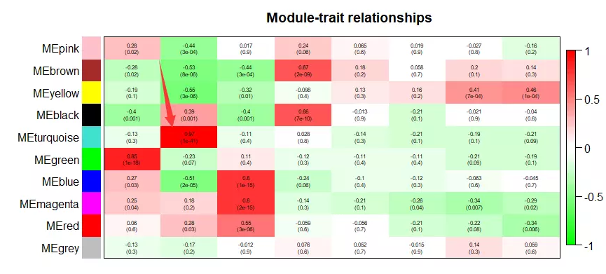

图中第二列第五行，即CB/turquoise相关性有0.97，pvalue=1e-41,后续分析可以挑选这个模块。
每一列对应的样本特征可以从design这里查看。

STEP6:感兴趣性状的模块的具体基因分析

下面就是对CB/turquoise这个模块具体分析：

首先计算模块与基因的相关性矩阵

# names (colors) of the modulesmodNames = substring(names(MEs), 3)
geneModuleMembership = as.data.frame(cor(datExpr, MEs, use = "p"));## 算出每个模块跟基因的皮尔森相关系数矩阵## MEs是每个模块在每个样本里面的值## datExpr是每个基因在每个样本的表达量MMPvalue = as.data.frame(corPvalueStudent(as.matrix(geneModuleMembership), nSamples));
names(geneModuleMembership) = paste("MM", modNames, sep="");
names(MMPvalue) = paste("p.MM", modNames, sep="");

再计算性状与基因的相关性矩阵

## 只有连续型性状才能只有计算## 这里把是否属于 CB 表型这个变量用0,1进行数值化。CB = as.data.frame(design[,2]);
names(CB) = "CB"geneTraitSignificance = as.data.frame(cor(datExpr, CB, use = "p"));
GSPvalue = as.data.frame(corPvalueStudent(as.matrix(geneTraitSignificance), nSamples));
names(geneTraitSignificance) = paste("GS.", names(CB), sep="");
names(GSPvalue) = paste("p.GS.", names(CB), sep="")

最后把两个相关性矩阵联合起来,指定感兴趣模块进行分析

module = "turquoise"column = match(module, modNames);
moduleGenes = moduleColors==module;
sizeGrWindow(7, 7);
par(mfrow = c(1,1));
verboseScatterplot(abs(geneModuleMembership[moduleGenes, column]),                   abs(geneTraitSignificance[moduleGenes, 1]),
                   xlab = paste("Module Membership in", module, "module"),
                   ylab = "Gene significance for CB",
                   main = paste("Module membership vs. gene significance\n"),
                   cex.main = 1.2, cex.lab = 1.2, cex.axis = 1.2, col = module)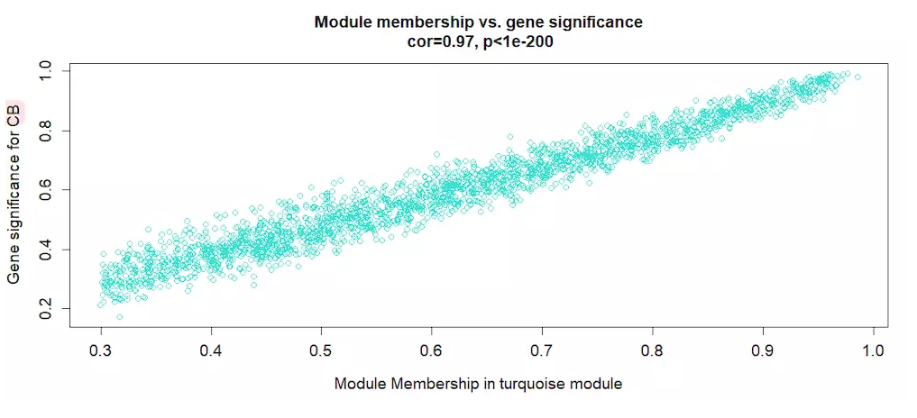

上图可以看出基因跟其对应的性状高度相关，可以导出做个GO/KEGG注释，看看这些基因的具体功能。

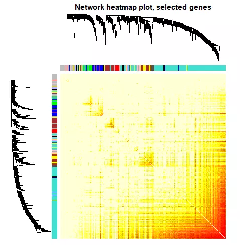
STEP7:网络的可视化

#首先针对所有基因画热图nGenes = ncol(datExpr)
nSamples = nrow(datExpr)
geneTree = net$dendrograms[[1]]; 
dissTOM = 1-TOMsimilarityFromExpr(datExpr, power = sft$powerEstimate); # 设置power=sft$powerEstimate，最佳beta值，此处是3plotTOM = dissTOM^7; 
diag(plotTOM) = NA; 
#TOMplot(plotTOM, geneTree, moduleColors, main = "Network heatmap plot, all genes")#然后随机选取部分基因作图nSelect = 400# For reproducibility, we set the random seedset.seed(10);
select = sample(nGenes, size = nSelect);
selectTOM = dissTOM[select, select];# There’s no simple way of restricting a clustering tree to a subset of genes, so we must re-cluster.selectTree = hclust(as.dist(selectTOM), method = "average")
selectColors = moduleColors[select];# Open a graphical windowsizeGrWindow(9,9)# Taking the dissimilarity to a power, say 10, makes the plot more informative by effectively changing# the color palette; setting the diagonal to NA also improves the clarity of the plotplotDiss = selectTOM^7;
diag(plotDiss) = NA;
TOMplot(plotDiss, selectTree, selectColors, main = "Network heatmap plot, selected genes")

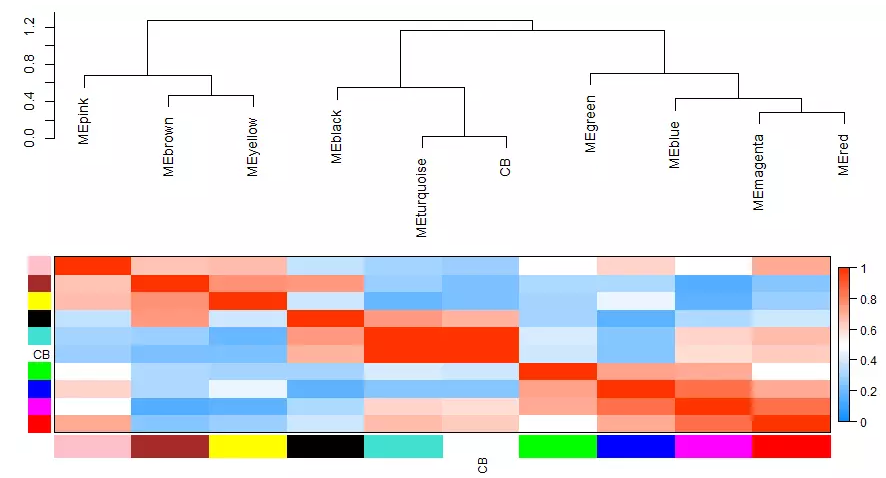
#最后画模块和性状的关系# Recalculate module eigengenesMEs = moduleEigengenes(datExpr, moduleColors)$eigengenes## 只有连续型性状才能只有计算## 这里把是否属于 Luminal 表型这个变量用0,1进行数值化。CB = as.data.frame(design[,2]);
names(CB) = "CB"# Add the weight to existing module eigengenesMET = orderMEs(cbind(MEs, CB))# Plot the relationships among the eigengenes and the traitsizeGrWindow(5,7.5);
par(cex = 0.9)
plotEigengeneNetworks(MET, "", marDendro = c(0,4,1,2), marHeatmap = c(3,4,1,2), cex.lab = 0.8, xLabelsAngle
                      = 90)# Plot the dendrogramsizeGrWindow(6,6);
par(cex = 1.0)## 模块的聚类图plotEigengeneNetworks(MET, "Eigengene dendrogram", marDendro = c(0,4,2,0),
                      plotHeatmaps = FALSE)# Plot the heatmap matrix (note: this plot will overwrite the dendrogram plot)par(cex = 1.0)## 性状与模块热图plotEigengeneNetworks(MET, "Eigengene adjacency heatmap", marHeatmap = c(3,4,2,2),
                      plotDendrograms = FALSE, xLabelsAngle = 90)

STEP8:提取指定模块的基因名

提取基因信息，进行下游分析包括GO/KEGG等功能数据库的注释。

# Select modulemodule = "turquoise";
# Select module probes
probes = colnames(datExpr) ## 我们例子里面的probe就是基因名
inModule = (moduleColors==module);
modProbes = probes[inModule];

GO分析

不知道这是gene ID类型，该怎么做注释呢？？？

STEP9: 模块的导出

主要模块里面的基因直接的相互作用关系信息可以导出到cytoscape,VisANT等网络可视化软件。

# Recalculate topological overlapTOM = TOMsimilarityFromExpr(datExpr, power = sft$powerEstimate); 
# Select modulemodule = "turquoise";# Select module probesprobes = colnames(datExpr) ## 我们例子里面的probe就是基因名inModule = (moduleColors==module);
modProbes = probes[inModule]; 
## 也是提取指定模块的基因名# Select the corresponding Topological OverlapmodTOM = TOM[inModule, inModule];
dimnames(modTOM) = list(modProbes, modProbes)

模块对应的基因关系矩阵

首先是导出到VisANT

vis = exportNetworkToVisANT(modTOM,
                            file = paste("VisANTInput-", module, ".txt", sep=""),
                            weighted = TRUE,
                            threshold = 0)

然后是导出到cytoscape

cyt = exportNetworkToCytoscape(
  modTOM,
  edgeFile = paste("CytoscapeInput-edges-", paste(module, collapse="-"), ".txt", sep=""),
  nodeFile = paste("CytoscapeInput-nodes-", paste(module, collapse="-"), ".txt", sep=""),
  weighted = TRUE,
  threshold = 0.02,
  nodeNames = modProbes, 
  nodeAttr = moduleColors[inModule]
);

STEP10: 模块内的分析—— 提取hub genes

• hub genes指模块中连通性（connectivity）较高的基因，如设定排名前30或前10%）。

• 高连通性的Hub基因通常为调控因子（调控网络中处于偏上游的位置），而低连通性的基因通常为调控网络中偏下游的基因（例如，转运蛋白、催化酶等）。
  HubGene: |kME| >=阈值（0.8）

模块特征相关的概念ME/kME/kIN ：

### Intramodular connectivity, module membership, and screening for intramodular hub genes

# (1) Intramodular connectivity

# moduleColors <- labels2colors(net$colors)
connet=abs(cor(datExpr,use="p"))^6Alldegrees1=intramodularConnectivity(connet, moduleColors)
head(Alldegrees1)

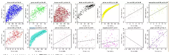
（2）模块内的连通性与gene显著性的关系

# (2) Relationship between gene significance and intramodular connectivitywhich.module="black"EB= as.data.frame(design[,2]); # change specific names(EB) = "EB"GS1 = as.numeric(cor(EB,datExpr, use="p"))GeneSignificance=abs(GS1)colorlevels=unique(moduleColors)sizeGrWindow(9,6)par(mfrow=c(2,as.integer(0.5+length(colorlevels)/2)))par(mar = c(4,5,3,1))for (i in c(1:length(colorlevels)))
{  whichmodule=colorlevels[[i]];
  restrict1 = (moduleColors==whichmodule);
  verboseScatterplot(Alldegrees1$kWithin[restrict1],
                     GeneSignificance[restrict1], col=moduleColors[restrict1],
                     main=whichmodule,
                     xlab = "Connectivity", ylab = "Gene Significance", abline = TRUE)
}

（3）计算模块内所有基因的连通性, 筛选hub genes
abs(GS1)> .9 可以根据实际情况调整参数
abs(datKME$MM.black)>.8 至少大于 >0.8

###(3) Generalizing intramodular connectivity for all genes on the arraydatKME=signedKME(datExpr, MEs, outputColumnName="MM.")# Display the first few rows of the data framehead(datKME)##Finding genes with high gene significance and high intramodular connectivity in# interesting modules# abs(GS1)> .9 可以根据实际情况调整参数# abs(datKME$MM.black)>.8 至少大于 >0.8FilterGenes= abs(GS1)> .9 & abs(datKME$MM.black)>.8
table(FilterGenes)

STEP11: 其他分析

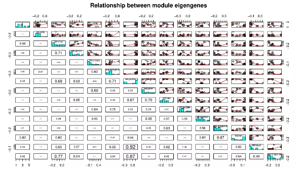
(1) another plot for realtionship between module eigengenes

plotMEpairs(MEs,y=datTraits$cellType)

(2) Diagnostics: heatmap plots of module expression
sizeGrWindow(8,9)

#par(mfrow=c(3,1), mar=c(1, 2, 4, 1))# for black modulewhich.module="blue";
plotMat(t(scale(datExpr[,moduleColors==which.module ]) ),nrgcols=30,rlabels=T,
        clabels=T,rcols=which.module,
        title=which.module )

（3） Diagnostics: displaying module heatmap and the eigengene

sizeGrWindow(8,7);
which.module="blue"ME=MEs[, paste("ME",which.module, sep="")]
par(mfrow=c(2,1), mar=c(0.3, 5.5, 3, 2))
plotMat(t(scale(datExpr[,moduleColors==which.module ]) ),
        nrgcols=30,rlabels=F,rcols=which.module,
        main=which.module, cex.main=2)
par(mar=c(5, 4.2, 0, 0.7))
barplot(ME, col=which.module, main="", cex.main=2,
        ylab="eigengene expression",xlab="MPP")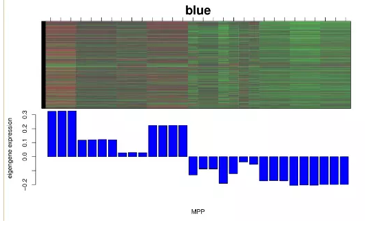

感谢Jimmy师兄和Aaron Li_bioinformatics师兄在学习过程中的指点。