Kintoki

Focus on machine learning, data mining, artificial intelligence

Enhanced learning (5)----- Time learning (Q learning, Sarsa learning)

Next, we review the characteristics of the dynamic programming algorithm (DP) and the Monte Carlo method (MC). The dynamic programming algorithm has the following characteristics:

• State transition probabilityPs aPsa

• The estimate of the state value function is bootstrapping , ie the update of the current state value function depends on other state value functions known.

In contrast, the characteristics of the Monte Carlo method are:

• You can learn from experience that you don't need an environment model

• Estimates of state value functions are independent of each other

• Can only be used for episode tasks

And the algorithm we want is this:

• No environment model required

• It is not limited to the episode task and can be used for continuous tasks.

This article describes the time difference study (Temporal-Difference learning, TD learning ) algorithm is provided with the above-described characteristics, which combines the MC and DP, and combines the advantages of the two algorithms.

TD Learing Thought

Before introducing TD learning, we first introduce the following simple Monte Carlo algorithm, which we call constant-ααMC , its state value function update formula is as follows:
 

V( st) ← V( st) + α [ Rt− V( st) ](1)(1)V(st)←V(st)+α[Rt−V(st)]

among themRtRtIs the actual cumulative return obtained after the end of each episode.ααIs the learning rate, the intuitive understanding of this formula is to use the actual cumulative returnRtRtAs a state value functionV( st)V(st)Estimated value . The specific approach is to examine each experiment in each episode.ststActual cumulative returnRtRtAnd current estimatesV( st)V(st)The deviation value, and multiply the deviation value by the learning rate to updateV( St)V(St)New valuation.

Now we will modify the formula as follows,RtRtChange tort + 1+ γV( st + 1)rt+1+γV(st+1), the TD (0) state value function update formula is obtained:
 

V( st) ← V( st) + α [ rt + 1+ γV( st + 1) − V( st) ](2)(2)V(st)←V(st)+α[rt+1+γV(st+1)−V(st)]

Why change to this form, we recall the definition of the state value function:
 

Vπ( s ) = Eπ[ r ( s‘| s,a)+γVπ( s‘) ](3)(3)Vπ(s)=Eπ[r(s‘|s,a)+γVπ(s‘)]

It is easy to find that this is actually based on the form of (3), using real immediate returnsrt + 1rt+1And the value function of the next stateV( st + 1)V(st+1)To updateV( st)V(st)This way is called the temporal difference. Since we do not have a state transition probability, multiple experiments are used to obtain the expected state value function estimate. Similar to the MC method, after enough experiments, the estimation of the state value function is able to converge to the true value.

So what is the difference between the MC and TD(0) update formulas? Let's take an example. Suppose there are the following eight episodes, where A-0 means that after passing state A, we get a return of 0:

Index	Samples
Episode 1	A-0, B-0
Episode 2	B-1
Episode 3	B-1
Episode 4	B-1
Episode 5	B-1
Episode 6	B-1
Episode 7	B-1
Episode 8	B-0

First we use constant-αα The MC method estimates the value function of state A, and the result isV( A ) = 0V(A)=0This is because state A only appears once in episode 1, and its cumulative return is zero.

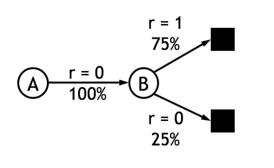
Now we use the update formula of TD(0), which is simple.λ = 1λ=1, we can getV( A ) = 0.75V(A)=0.75. How is this result calculated? First, the value function of state B is easy to find, and B is the termination state, and the probability of getting a return of 1 is 75%, soV( B ) = 0.75V(B)=0.75. Then from the data we can get the probability that state A is transferred to state B is 100% and the return is 0. According to formula (2)V( A ) ← V( A ) + α [ 0 + λ V( B ) − V( A ) ]V(A)←V(A)+α[0+λV(B)−V(A)]Visible in onlyV( A ) = λ V( B ) = 0.75V(A)=λV(B)=0.75At the time, equation (2) converges. For this example, it can be plotted:

Visibility (2) is more reasonable because it can take advantage of other state estimates, and since it does not need to wait until the end of the task to update the estimate, it is no longer limited to episode. Task. In addition, experiments show that TD(0) is also significantly better than the MC method in terms of convergence rate.

After using equation (2) as the estimation formula of the state value function, the strategy estimation algorithm introduced in the previous article becomes the following form. This algorithm is called TD prediction:

Input: Strategy to be estimatedππ
Initialize all arbitrarilyV( s )V(s), (e . g. , V( s ) = 0 , ∀ s ∈ s+e.g.,V(s)=0,∀s∈s+)
Repeat (for all episode):
initialization statess
Repeat (for each step state transition):
a ←a←StrategyππLower statessTake action
take actionaaObserving returnsrr, and the next states‘s‘
V( s ) ← V( s ) + α [ r + λ V( s‘) − V( s ) ]V(s)←V(s)+α[r+λV(s‘)−V(s)]
s ← s‘s←s‘
UntilststIs terminal
Until allV( s )V(s)Convergence
outputVπ( s )Vπ(s)

Sarsa algorithm

Now we use TD prediction to form a new reinforcement learning algorithm that is used in decision/control problems. Here, the reinforcement learning algorithm can be divided into two types: on-policy and off-policy . The sarsa algorithm to be introduced first belongs to the on-policy algorithm.
A little different from the previous DP method, the sarsa algorithm estimates the action value function (Q function) instead of the state value function. In other words, we estimate the strategyππAny statessAction value function for all executable actions aQπ( s , a )Qπ(s,a)The Q function can also be estimated using the TD Prediction algorithm. The following is a fragment of the state-action pair sequence and the corresponding reward value.

Give the sarsa action value function update formula as follows:
 

Q ( st, at) ← Q ( st, at) + α [ rt + 1+ λ Q ( st + 1, at + 1) − Q ( st, at) ](4)(4)Q(st,at)←Q(st,at)+α[rt+1+λQ(st+1,at+1)−Q(st,at)]

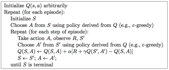
It can be seen that the formula (4) is basically the same as the form of the formula (2). Note that for each non-terminating statestst, in the next statest + 1st+1After that, you can use the above formula to updateQ ( st, At)Q(st,At)And ifststIs the termination state, then it is necessaryQ ( st + 1= 0 , at + 1)Q(st+1=0,at+1). Since each update of the action value function is( st, at, rt + 1, st + 1, at + 1)(st,at,rt+1,st+1,at+1)Correlation, so the algorithm is named sarsa algorithm. The complete flow chart of the sarsa algorithm is as follows: the

algorithm finally obtains the Q function of all state-action pairs, and outputs the optimal strategy according to the Q function.ππ

Q-learning

In sarsa algorithm, the strategy to follow when selecting actions and policies followed in the value of the function updates the action is the same, that is,ε − gr e e dyε−greedyThe strategy, and in the Q-learning introduced next, the action value function update is different from the strategy that is followed when selecting the action . This method is called Off-Policy . The Q-learning action value function update formula is as follows:
 

Q ( st, at) ← Q ( st, at) + α [ rt + 1+ λ maxaQ ( st + 1, a ) − Q ( st, at) ](5)(5)Q(st,at)←Q(st,at)+α[rt+1+λMaxaQ(st+1,a)−Q(st,at)]

It can be seen that the biggest difference between Q-learning and sarsa algorithm is that when the Q value is updated, the largest one is used directly.Q ( st + 1, a )Q(st+1,a)Value - equivalent to the useQ ( st + 1, a )Q(st+1,a)The action with the largest value, and the currently executed strategy, that is, the action selectedatatThe strategy used at the time is irrelevant.The Off-Policy method simplifies the difficulty of proving algorithm analysis and proof of convergence, and its convergence is proved very early. The complete flow chart of Q-learning is as follows:

 

summary

This article introduces the TD method idea and the TD(0), Q(0), and Sarsa(0) algorithms. The TD method combines the advantages of Monte Carlo method and dynamic programming, can be applied to model-free, continuous tasks, and has excellent performance, so it has been well developed, and Q-learning has become a reinforcement learning. The most widely used method. In the next article, we will introduce Eligibility Traces to improve the performance of the algorithm. After combining Eligibility Traces, we can getQ ( λ ) , Sa r s a ( λ )Q(λ),Sarsa(λ)Algorithm

Reference material

[1] R. Sutton et al. Reinforcement learning: An introduction, 1998